Note

Please report issues with the manual on the GitHub page.

9.1.4. Urban Energy Balance - SUEWS and WUDAPT

9.1.4.1. Introduction

Note

This tutorial is not ready for use. Work in progress.

In this tutorial you will generate input data for the SUEWS model and simulate spatial (and temporal) variations of energy exchanges within an area in New York City using local climate zones derived within the WUDAPT project. The World Urban Database and Access Portal Tools project is a community-based project to gather a census of cities around the world.

Note

This tutorial is currently designed to work with QGIS 2.18. It is strongly recommended that you goo through the Urban Energy Balance - SUEWS Spatial tutorial before you go through this tutrial.

9.1.4.2. Objectives

To prepare input data for the SUEWS model using a WUDAPT dataset and analyse energy exchanges within an area in New York City, US.

9.1.4.3. Initial Steps

UMEP is a python plugin used in conjunction with QGIS. To install the software and the UMEP plugin see the getting started section in the UMEP manual.

As UMEP is under development, some documentation may be missing and/or there may be instability. Please report any issues or suggestions to our repository.

9.1.4.3.1. Loading and analyzing the spatial data

Note

You can download the all the data from here. Unzip and place in a folder where you have read and write access to. The LCZ data for various cities are also available from the WUDAPT portal.

• Start by loading the raster dataset (NYC_LCZ.tif) into an empty QGIS project. This dataset is referenced to the WGS84 CRS (ESPG:4326).

• You can set the correct colors for your LCZ raster by opening the LCZ converter at UMEP > Pre-Processer > Spatial data > LCZ converter. In the upper right corner, choose the LCZ raster and press Color Raster and then close the LCZ Converter.

9.1.4.4. Vector grid generation

A vector polygon grid is required for specifying the extent and resolution of the modelling.You will make use of a built-in tool in QGIS to generate such a grid.

1. First zoom in to Manhattan as shown in the figure below

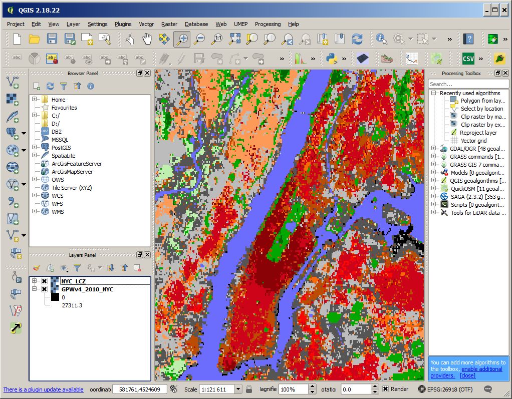
Fig. 9.23 Zoom in the Manhattan island.

1. As WGS84 (EPSG:4326) is in degree coordinates and maybe you want to specify your grid in meters, you need to change the CRS of your current QGIS-project. Click on the globe at the bottom right of your QGIS window and select ESPG:26918 as your ‘on the fly’ CRS.

2. Open vector grid at Vector > Research Tools > Vector grid.

3. Select the extend of your canvas by clicking the … next to Grid extent (xmin, xmax, ymin, ymax) and select Use layer/canvas extent.

4. Select Use Canvas Extent.

5. As you can see the units in now in meters and not in degrees. Specify the desired grid spacing to 5000 meters. This will save time later on. Of course you can set it a much smaller number if you have the time to wait when the model performs the calculations later on.

6. Make sure the output is in polygons, not lines.

7. Create as temporary layer.

8. Save your grid by right-click on the new layer in the Layers Panel and choose Save as…. Here it is very imporant that you save in the same CRS as you other layers (ESPG:4326). Save as a shape file.

9.1.4.5. Population density

Population density is required to estimate the anthropogenic heat release (Q_F) in SUEWS. There is a possibility to make use of both night-time and daytime population densities to make the model more dynamic. In this tutorial you will only use a night-time dataset. This dataset can be aqcuired from the Spatial Data Downloader in UMEP.

1. Open de spatial downloader at UMEP > Pre-Processer > Spatial data > Spatial Data Downloader.

2. Select population density and select the GPWv4: UN-Adjusted Population Density closest to the year you intend to model (2010). The values will be in (pp / square kilometer).

3. Make sure your canvas is zoomed out to the entire LCZ map and click Use canvas extent

4. Now click Get data.

5. Save as a geoTiff (.tif) with the name GPWv4_2010.

6. Now you need to calculate population density per grid in units pp/hectare. First open the QGIS built-in tool Zonal statistics (Raster > Zonal Statistics). If the tool is absent you need to activate it by going to Plugins > Manage and Install Plugins and add Zonal statistics plugin. Open the tool and make the settings as shown below. This will calulate mean population density per grid.

   

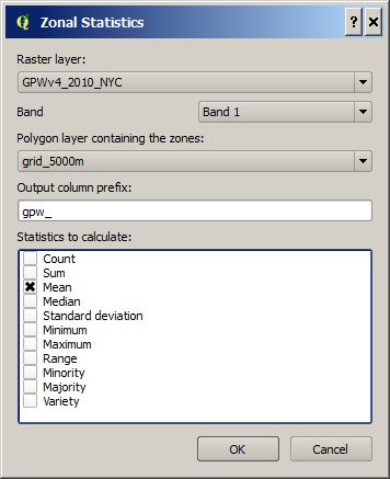
   Fig. 9.24 Settings for the Zonal statistics plugin.

7. Open the attribute table for your Grid_5000m-layer (right-click on layer and choose (Open attribute Table).

8. Click the abacus shaped symbol this is the Field calculator.

9. Under Output field name write “pp_ha, the Output field type should be “Decimal number (real)”, and the Output Precision can be set to 2.

10. In the expression dialog box write gpw_mean/100, here gpw_mean is the name of your population density field and the 100 is to convert the data from km² to ha.

11. Click OK and you should have a new field called “pp_ha”.

12. Click the yellow pencil in the top left corner of the attribute table to stop editing and save your changes and close the attribute table.

9.1.4.6. LCZ converter

Now you will make use of the LCZ Converter-plugin to generate input data for the SUEWS model.

1. Open the LCZ converter at UMEP > Pre-Processer > Spatial data > LCZ converter.

2. Select the LCZ raster layer at ‘’ LCZ raster’‘.

3. Select the vector grid you have just created in step 3 at Vector grid and select the ID field of the polygon grid at ID field.

4. By clicking Adjust default parameters you can edit the table. This table specifies the pervious, trees, grass, etc. fractions for each of the LCZ classes. For more information about each of the classes see LCZConverter. If you choose to edit the table, make sure all fractions add up to 1.0.

5. If you are unsure about the exact fractions for each of the LCZ click the tab Pervious distribution. Select Same for all LCZ’s

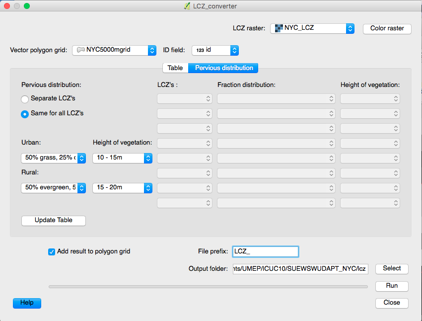
Fig. 9.25 Settings for the LCZ converter plugin.

1. Now you can select your best estimate about the distribution of the pervious surface fractions for urban and the tree distribution for rural. In addition, also specify the expected height of the trees.

2. Once you are satisfied click Update Table.

3. Select add results to polygon.

4. Add a file prefix if desired.

5. Finally select an output folder where you would like to receive the text files and click Run.

Note

For mac users use this workaround: manually create a directory, go into the folder above and type the folder name. It will give a warning “—folder name–” already exists. Do you want to replace it? Click replace.

This should generate 3 text files, one with the land cover fractions, one with morphometric parameters for buildings and one for trees for each grid cell of the polygon grid.

9.1.4.7. SUEWS

Before running SUEWS, you will need to prepare some of the data required to run it.

1. SUEWS prepare requires the grid CRS to be in metres not degrees, therefore we need to reproject the grid. Right-click the vector grid and click save as... Assign a different file name, use CRS ESPG:26918 and click OK.

2. Open SUEWS prepare at: UMEP > Pre-Processer > SUEWS prepare.

3. Under vector polygon grid specify your reprojected vector grid and the ID field.

4. Select the location of the Meteorological file that was included in the input data, the building morphology (_build_), tree morphology (_veg_) and land cover fractions (_LCFGrid_) from the step above and the population density (pp_ha) in the dropdown list.

5. Enter the start and end of day light savings time for 2010 and the UTC offset of New York.

6. Specify the Leaf cycle = winter when initialising in January. Unless the user has better information initialise the Soil moisture state at 100 %.

7. Select an output folder where the initial data to run SUEWS should be saved and press Generate.

8. Open SUEWS at UMEP > Processer > Urban Energy Balance > Urban Energy Balance (SUEWS/BLUEWS, advanced). Using this for the first time, the system will ask you to download the latest version of SUEWS, click OK.

9. Change the OHM option to [1]. This allows the anthropogenic energy to be partitioned also into the storage energy term.

10. Leave the rest of the combobox settings at the top as default and tick both the Use snow module and the Obtain temporal resolution… box.

11. Set the Temporal resolution of output (minutes) to 60.

12. Locate the directory where you saved your output from SUEWSPrepare earlier and choose an output folder of your choice.

13. Also, Tick the box Apply spin-up using…. This will force the model to run twice using the conditions from the first run as initial conditions for the second run.

14. Click Run. This computation will take a while so be patient. If it only takes a very short time (a few seconds) the model has probably crashed. Please consult the problems.txt file for more information.

9.1.4.8. Analysing model reults

When the model has successfully run, it is time to look at some of the output of the model. The SUEWSAnalyser tool is available from the post-processing section in UMEP.

1. To better visualise what would be interesting to plot, label the grid ID’s of your vector grid. Do this by right-clicking the vector grid, going to properties, under the Labels tab click Show labels for this layer, label with id and select a text format of your choosing.

2. Open UMEP > Post-Processor > Urban Energy Balance > SUEWS Analyzer. There are two main sections in this tool. The Plot data-section can be used to make temporal analysis as well as making simple comparisins between two grids or variables. This Spatial data-section can be used to make aggregated maps of the output variables from the SUEWS model. This requires that you have loaded the same polygon grid into your QGIS project that was used when you prepared the input data for SUEWS using SUEWS Prepare earlier in this tutorial.

3. To access the output data from the a model run, the RunControl.nml file for that particular run must be located. If your run has been made through UMEP, this file can be found in your output folder. Otherwise, this file can be located in the same folder from where the model was executed. In the top panel of SUEWS Analyzer, load the RunControl.nml located in the output folder.

Feel free to try plotting different variables, first let’s try and look at a variable for two different grid cells.

1. Load the RunControl.nml located in the output folder.

2. On the left hand specify a Grid cell that is largely urban, select Year to investigate. Select the desired time period and a variable, for example Sensible heat flux.

3. Comparing with another less urbanised gridcell turn on include another variable and specify the desired Grid, selecting the same Variable (Sensible heat flux).

4. Click plot.

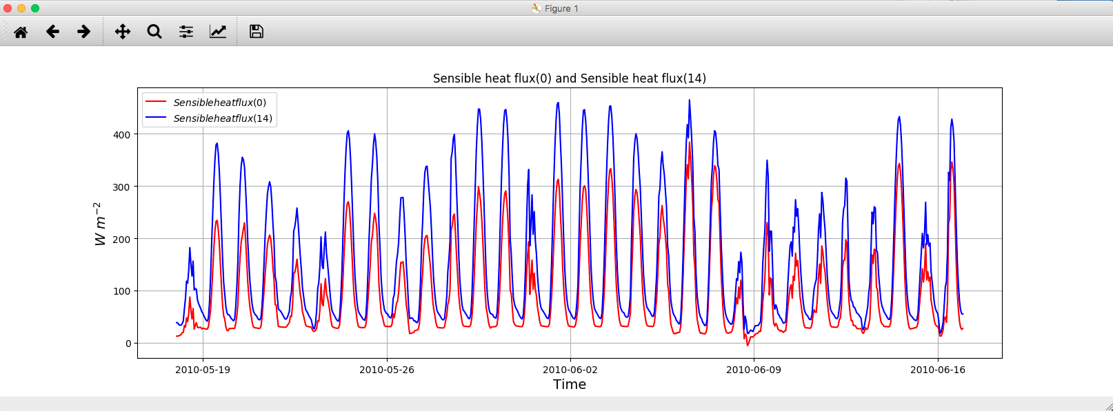
Fig. 9.26 Example of the comparison of the heat flux for two grid cell in the vector grid.

Now we will look at the horizontal distribution of the storage flux. #. On the right-hand side of SUEWS analyser specify the Net Storage flux as a variable to analyse. #. Select the Year to investigate and a time period during the summer season. #. Select the Median and Only daytime. #. Select the Vector polygon grid you have been using and save as a GeoTiff. #. Specify an output filename, and tick Add Geotiff to map canvas and Generate.

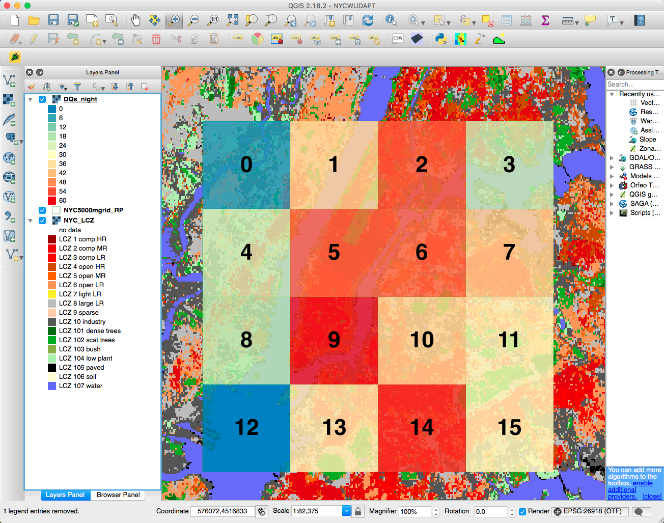
Fig. 9.27 Example of the median, night-time net storage flux.

This should generate a geotiff file with a median, night-time net storage flux in the selected timeperiod.

Tutorial finished.