Tip

1. Need help? Please let us know in the UMEP Community.

2. Please report issues with the manual on the GitHub Issues.

3. Please cite SUEWS with proper information from our Zenodo page.

1. Parameterisations and sub-models within SUEWS

1.1. Net all-wave radiation, Q*

There are several options for modelling or using observed radiation components depending on the data available. As a minimum, SUEWS requires incoming shortwave radiation to be provided.

1. Observed net all-wave radiation can be provided as input instead of being calculated by the model.

2. Observed incoming shortwave and incoming longwave components can be provided as input, instead of incoming longwave being calculated by the model.

3. Other data can be provided as input, such as cloud fraction (see options in RunControl.nml).

4. NARP (Net All-wave Radiation Parameterization) [Loridan et al., 2011, Offerle et al., 2003] scheme calculates outgoing shortwave and incoming and outgoing longwave radiation components based on incoming shortwave radiation, temperature, relative humidity and surface characteristics (albedo, emissivity).

5. SPARTACUS-Surface (SS) computes the 3D interaction of shortwave and longwave radiation with complex surface canopies, including vegetated and urban canopies (with or without vegetation). More details can be found in the SPARTACUS-Surface (SS) section.

1.2. Anthropogenic heat flux, Q_F

1. Two simple anthropogenic heat flux sub-models exist within SUEWS:

   • Järvi et al. [2011] approach, based on heating and cooling degree days and population density (allows distinction between weekdays and weekends).

   • Loridan et al. [2011] approach, based on a linear piece-wise relation with air temperature.

2. Pre-calculated values can be supplied with the meteorological forcing data, either derived from knowledge of the study site, or obtained from other models, for example:

   • LUCY [Allen et al., 2010, Lindberg et al., 2013]. A new version has been now included in UMEP. To distinguish it is referred to as LQF

   • GreaterQF [Iamarino et al., 2011]. A new version has been now included in UMEP. To distinguish it is referred to as GQF

1.3. Storage heat flux, ΔQ_S

1. Three sub-models are available to estimate the storage heat flux:

   • OHM (Objective Hysteresis Model) [Grimmond and Oke, 1999, Grimmond and Oke, 2002, Grimmond et al., 1991]. Storage heat heat flux is calculated using empirically-fitted relations with net all-wave radiation and the rate of change in net all-wave radiation.

   • AnOHM (Analytical Objective Hysteresis Model) [Sun et al., 2017]. OHM approach using analytically-derived coefficients. Not recommended in this version.

   • ESTM (Element Surface Temperature Method) [Offerle et al., 2005]. Heat transfer through urban facets (roof, wall, road, interior) is calculated from surface temperature measurements and knowledge of material properties. Not recommended in this version.

2. Alternatively, ‘observed’ storage heat flux can be supplied with the meteorological forcing data.

1.4. Turbulent heat fluxes, Q_H and Q_E

1. LUMPS (Local-scale Urban Meteorological Parameterization Scheme) [Grimmond and Oke, 2002] provides a simple means of estimating sensible and latent heat fluxes based on the proportion of vegetation in the study area.

2. SUEWS adopts a more biophysical approach to calculate the latent heat flux; the sensible heat flux is then calculated as the residual of the energy balance. The initial estimate of stability is based on the LUMPS calculations of sensible and latent heat flux. Future versions will have alternative sensible heat and storage heat flux options.

Sensible and latent heat fluxes from both LUMPS and SUEWS are provided in the Output files. Whether the turbulent heat fluxes are calculated using LUMPS or SUEWS can have a major impact on the results. For SUEWS, an appropriate surface conductance parameterisation is also critical [Järvi et al., 2011] [Ward et al., 2016]. For more details see Differences_between_SUEWS_LUMPS_and_FRAISE .

1.5. Water balance

The running water balance at each time step is based on the urban water balance model of Grimmond et al. [1986] and urban evaporation-interception scheme of Grimmond and Oke [1991].

• Precipitation is a required variable in the meteorological forcing file.

• Irrigation can be modelled [Järvi et al., 2011] or observed values can be provided if data are available.

• Drainage equations and coefficients to use must be specified in the input files.

• Soil moisture can be calculated by the model.

• Runoff is permitted:

  • between surface types within each model grid

  • between model grids (Not available in this version.)

  • to deep soil

  • to pipes.

1.6. Snowmelt

The snowmelt model is described in Järvi et al. [2014]. Changes since v2016a: 1) previously all surface states could freeze in 1-h time step, now the freezing surface state is calculated similarly as melt water and can freeze within the snow pack. 2) Snowmelt-related coefficients have also slightly changed (see SUEWS_Snow.txt).

1.7. Convective boundary layer

A convective boundary layer (CBL) slab model [Cleugh and Grimmond, 2001] calculates the CBL height, temperature and humidity during daytime [Onomura et al., 2015].

1.8. Wind, Temperature and Humidity Profiles in the Roughness Sublayer

A dignostic RSL scheme for calculating the wind, temperature and humidity profiles in the roughness sublayer is implemented in 2020a following Harman and Finnigan [2007], Harman and Finnigan [2008] and Theeuwes et al. [2019]. An recent application of this RSL scheme can be found in Tang et al. [2021].

The diagnostic profiles are outputed in 30 uneven levels between the ground and forcing height, which are divided into two groups:

• One group of levels are evenly distributed within the urban canopy layer characterised by mean height of roughness elements (e.g. buildings, trees, etc.) \(z_H\), which determines the number of layers within urban canopy \(n_{can}\):

\[ n_{can} = \begin{cases} 3 & \text{if } z_H \leq \text{2 m} \\ 10 & \text{if } \text{2 m} \lt z_H \leq \text{10 m} \\ 15 & \text{if } z_H \gt \text{10 m} \\ \end{cases} \]

• The other levels are evenly distributed between the urban canopy layer top and forcing height.

Note

All the diagnostic profiles (wind speed, temperature and humidity) are calculated from the forcing data down into the canopy. Therefore it is assumed that the forcing temperature and humidity are above the blending height.

Common near-surface diagnostics:

• T2: air temperature at 2 m agl

• Q2: air specific humidity at 2 m agl

• RH2: air relative humidity at 2 m agl

• U10: wind speed at 10 m agl

are calculated by the RSL scheme by interpolating RSL profile results to the corresponding diagnostic heights.

1.9. SPARTACUS-Surface (SS)

Warning

This module is highly experimental and not yet fully tested: description here is not yet complete, either. Please refer to the original SPARTACUS-Surface page for more details, which may differ from the coupled version in SUEWS described below due to possibly different implementations.

Note

Future Work

• New SUEWS input table containing SPARTACUS profiles

• Add check for consistency of SUEWS and SS surface fractions

• Include snow

1.9.1. Introduction to SS

The SPARTACUS-Surface module computes the 3D interaction of shortwave and longwave radiation with complex surface canopies, including vegetated and urban canopies (with or without vegetation).

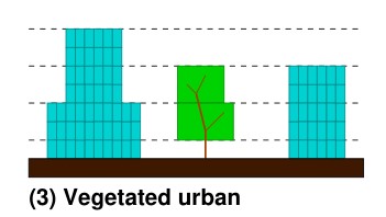
Fig. 1.1 Multi-layer structure (horizontal dashed lines) used in SS to characterise differences in the canopy (Cyan building, Green – vegetation). Source: SPARTACUS-Surface GH page

It uses a multi-layer description of the canopy (Fig. 1.1), with a statistical description of the horizontal distribution of trees and buildings. Assumptions include:

• Trees are randomly distributed.

• Wall-to-wall separation distances follow an exponential probability distribution.

• From a statistical representation of separation distances one can determine the probabilities of light being intercepted by trees, walls and the ground.

In the tree canopy (i.e. between buildings) there are two or three regions (based on user choice) (Fig. 1.2): clear-air and either one vegetated region or two vegetated regions of equal fractional cover but different extinction coefficient. Assumptions include:

• The rate of exchange of radiation between the clear and vegetated parts of a layer are assumed to be proportional to the length of the interface between them.

• Likewise for the rate of interception of radiation by building walls.

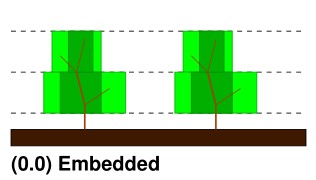
Fig. 1.2 Areas between trees. Source: SPARTACUS-Surface GH page

Each time light is intercepted it can undergo diffuse or specular reflection, be absorbed or be transmitted (as diffuse radiation). The probabilities for buildings and the ground are determined by albedos and emissivities, and for trees are determined by extinction coefficients and single scattering albedos.

1.9.2. SUEWS-SS Implementation

• Maximum of 15 vertical layers.

• Building and tree fractions, building and tree dimensions, building albedo and emissivity, and diffuse versus specular reflection, can be treated as vertically heterogenous or uniform with height depending on parameter choices.

• As tree fraction increases towards 1 it is assumed that the tree crown merges when calculating tree perimeters.

• Representing horizontal heterogeneity in the tree crowns is optional. When represented it is assumed that heterogeneity in leaf area index is between the core and periphery of the tree, not between trees.

• When calculating building perimeters it is assumed that buildings do not touch (analogous to crown shyness) as building fraction increases towards 1.

• Vegetation extinction coefficients (calculated from leaf area index, LAI) are assumed to be the same in all vegetated layers.

1

Confirming the ESTM coupling will allow this to be modified.

• Building facet and ground temperatures are equal to SUEWS TSfc_C (i.e.surface temperature) 1.

2

It is the forcing air temperature not RSL temperature. Future developments might make leaf temperature change with height.

• Leaf temperatures are equal to SUEWS temp_C (i.e. air temperature within the canopy) 2.

• Ground albedo and emissivity are an area weighted average of SUEWS paved, grass, bare soil and water values.

• Inputs from SUEWS: sfr, zenith_deg, TSfc_C, avKdn, ldown, temp_c, alb_next, emis, LAI_id.

• SS specific input parameters: read in from SUEWS_SPARTACUS.nml.

• Outputs used by SUEWS: alb_spc, emis_spc, lw_emission_spc.

• Although the radiation is calculated in multiple vertical layers within SS it is only the upwelling top-of-canopy fluxes: alb_spc*avKdn, (emis_spc)*ldown, and lw_emission_spc that are used by SUEWS.

3

this will be updated but requires other updates first as of December 2021

• Output variables (including multi-layer ones) are in SUEWS-SS output file SSss_YYYY_SPARTACUS.txt. 3

1.9.3. RSL and SS Canopy Representation Comparison

• The RSL has 30 levels but when the average building height is <2 m, < 12 m and > 12 m there are 3, 10 and 15 evenly spaced layers in the canopy.

• The remaining levels are evenly spaced up to the forcing level (Fig. 1.3).

• The buildings are assumed to be uniform height.

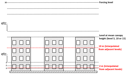
Fig. 1.3 SUEWS-RSL module assumes the RSL has 30 layers that are spread between the canopy and within the atmosphere above

A maximum of 15 layers are used by SS (vertial_layers_SS-RSL), with the top of the highest layer at the tallest building height. The layer heights are user defined and there is no limit on maximum building height. The buildings are allowed to vary in height.

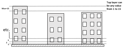
Fig. 1.4 Vertical layers used by SS

1.9.4. How to use SUEWS-SS

1.9.4.1. Inputs

To run SUEWS-SS the SS specific files that need to be modified are:

• RunControl.nml (see NetRadiationMethod)

• SUEWS_SPARTACUS.nml

Note

Non-SS specific SUEWS input file parameters also need to have appropriate values. For example, LAI, albedos and emissivities are used by SUEWS-SS as explained in More background information.

1.9.4.2. Outputs

See SSss_YYYY_SPARTACUS_TT.txt.

1.9.5. More background information

1.9.5.1. Vegetation single scattering albedo (SSA)

The shortwave broadband SSA is equal to the sum of the broadband reflectance \(R\) and broadband transmittance \(T\) [Yang et al., 2020]. Given reflectance \(r\) and transmittance \(t\) spectra the SSA is calculated to modify equation

\[\text{SSA} = \ \frac{\int_{\sim 400\ \text{nm}}^{\sim 2200\ \text{nm}}{r \times S}\text{dλ}}{\int_{\sim 400\ \text{nm}}^{\sim 2200\ \text{nm}}S\text{dλ}} + \frac{\int_{\sim 400\ \text{nm}}^{\sim 2200\ \text{nm}}{t \times S}\text{dλ}}{\int_{\sim 400\ \text{nm}}^{\sim 2200\ \text{nm}}S\text{dλ}}\]

where \(S\) clear-sky surface spectrum :numfig:`rami5`.

The integrals are performed between 400 nm and 2200 nm because this is the spectral range that RAMI5⁵ Järvselja birch stand forest spectra are available. This is a reasonable approximation since it is where the majority of incoming SW energy resides (as seen from the clear-sky surface spectrum in Fig. 6).

Users can use the default value of 0.46, from RAMI5 Järvselja birch stand forest tree types or calculate their own SSA (Fig. 1.5). There are more tree R and T profiles here⁵,

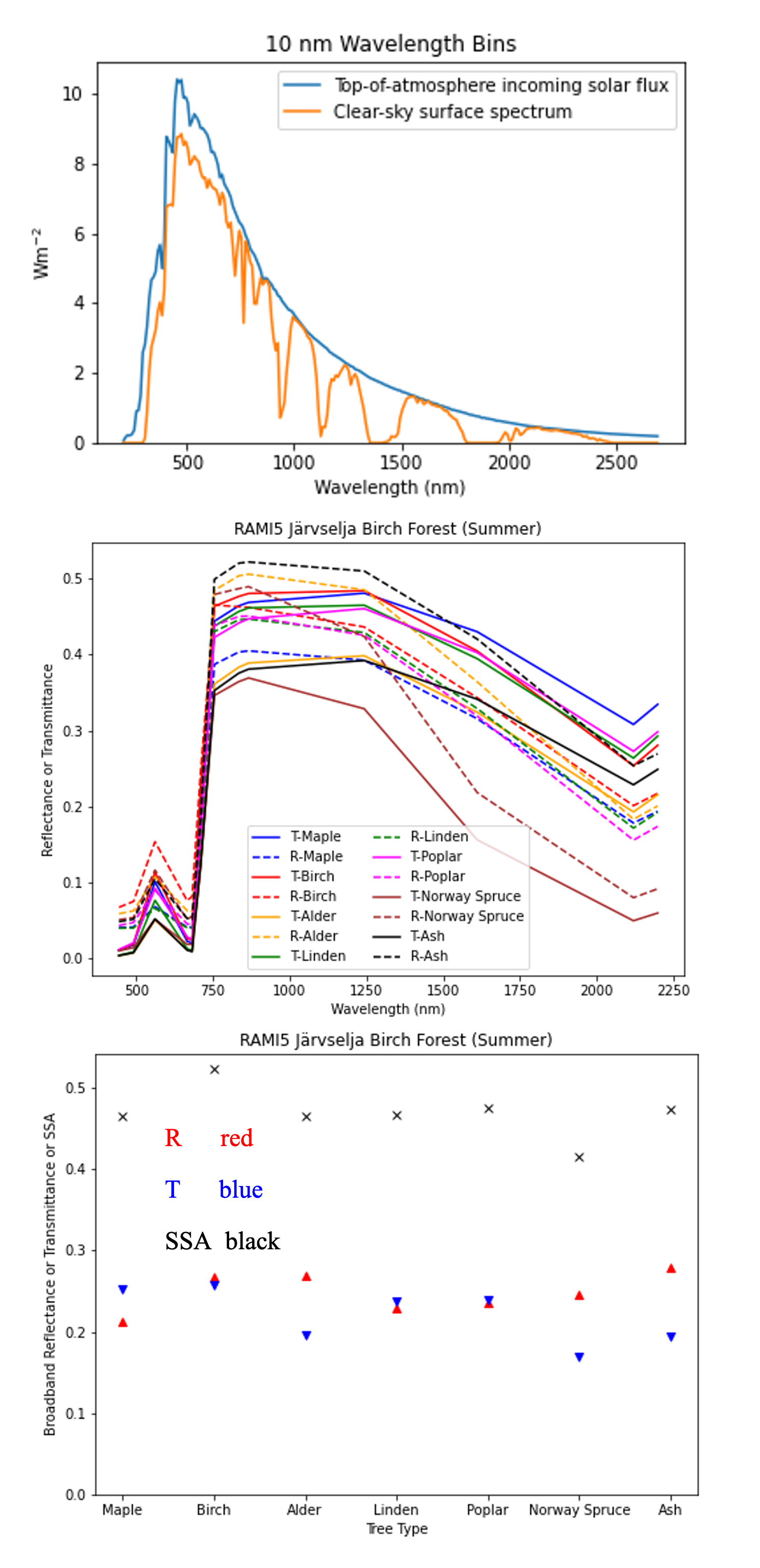
Fig. 1.5 RAMI5⁵ data used to calculate R, T, and SSA, and R, T, and SSA values: (a) top-of-atmosphere incoming solar flux and clear-sky surface spectrum [Hogan and Matricardi, 2020] (b) RAMI5 r and t spectra, and (c) calculated broadband R, T, and SSA values.

The longwave broadband SSA could be calculated in the same way but with the integral over the thermal infra-red (8-14 𝜇m), S replaced with the Plank function at Earth surface temperature, and r and t for the spectra for the thermal infra-red. The approximation that R + T = 2R can be made. r for different materials is available at https://speclib.jpl.nasa.gov/library. The peak in the thermal infra-red is ~10 𝜇m. Based on inspection of r profiles for several tree species SSA=0.06 is the default value.

1.9.5.2. Building albedo and emissivity

Use broadband values in Table C.1 of Kotthaus et al. [2014]. Full spectra can be found in the spectral library documentation.

1.9.5.3. Ground albedo and emissivity

In SUEWS-SS this is calculated as:

(𝛼(1)*sfr(PavSurf)+𝛼(5)*sfr(GrassSurf)+𝛼(6)*sfr(BSoilSurf)+𝛼(7)*sfr(WaterSurf))/ (sfr(PavSurf) + sfr(GrassSurf) + sfr(BSoilSurf) + sfr(WaterSurf))

where 𝛼 is either the ground albedo or emissivity.

𝛼 values for the surfaces should be set by specifying surface codes in SUEWS_SiteSelect.txt. Codes should correspond to existing appropriate surfaces in SUEWS_NonVeg.txt and SUEWS_NonVeg.txt. Alternatively, new surfaces can be made in SUEWS_NonVeg.txt and SUEWS_NonVeg.txt with 𝛼 values obtained for example from the spectral library.

1.9.5.4. Consistency of SUEWS and SS parameters

SUEWS building and tree (evergreen+deciduous) fractions in SUEWS_SiteSelect.txt should be consistent with the SUEWS_SPARTACUS.nml building_frac and veg_frac of the lowest model layer.

1.9.5.5. Leaf area index (LAI)

The total vertically integrated LAI provided by SUEWS is used in SS to determine the LAI and vegetation extinction coefficient in each layer. Surface codes in SUEWS_SiteSelect.txt should correspond to appropriate LAI values in SUEWS_Veg.txt.