Note
Please report issues with the manual on the GitHub page.
9.1. Urban Energy Balance - SUEWS Introduction
9.1.1. Introduction
In this tutorial you will use a land-surface model, SUEWS to simulate energy exchanges in a city (London is the test case).
SUEWS (Surface Urban Energy and Water Balance Scheme) allows the energy and water balance exchanges for urban areas to be modelled (Järvi et al. 2011, 2014, Ward et al. 2016a). The model is applicable at the neighbourhood scale (e.g. 102 to 104 m). The fluxes calculated are applicable to height of about 2-3 times the mean height of the roughness elements; i.e. above the roughness sublayer (RSL). The use of SUEWS within Urban Multi-scale Environmental Predictor (UMEP) provides an introduction to the model and the processes simulated, the parameters used and the impact on the resulting fluxes.
Tools such as this, once appropriately assessed for an area, can be used for a broad range of applications. For example, for climate services (e.g. http://www.wmo.int/gfcs/). Running a model can allow analyses, assessments, and long-term projections and scenarios. Most applications require not only meteorological data but also information about the activities that occur in the area of interest (e.g. agriculture, population, road and infrastructure, and socio-economic variables).
Model output may be needed in many formats depending on a users’ needs. Thus, the format must be useful, while ensuring the science included within the model is appropriate. The figure below provides an overview of UMEP, a city based climate service tool (CBCST). Within UMEP there are a number of models which can predict and diagnose a range of meteorological processes. In this activity we are concerned with SUEWS, initially the central components of the model. See manual or published papers for more detailed information of the model.
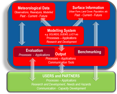
Fig. 9.1 Overview of the climate service tool UMEP (from Lindberg et al. 2018)
SUEWS can be run in a number of different ways:
- Within UMEP via the Simple selection. This is useful for becoming familiar with the model (Part 1)
- Within UMEP via the Advanced selection. This can be used to exploit the full capabilities of the model (Part 2)
- SUEWS standalone (see manual)
- Within other larger scale models (e.g. WRF).
9.1.2. SUEWS Simple Objectives
This tutorial introduces SUEWS and demonstartes how to run the model within UMEP (Urban Multi-scale Environmental Predictor). Help with Abbreviations.
9.1.2.1. Steps
- An introduction to the model and how it is designed.
- Different kinds of input data that are needed to run the model
- How to run the model
- How to examine the model output
9.1.3. Initial Steps
UMEP is a python plugin used in conjunction with QGIS. To install the software and the UMEP plugin see the getting started section in the UMEP manual.
As UMEP is under development, some documentation may be missing and/or there may be instability. Please report any issues or suggestions to our repository.
9.1.4. SUEWS Model Inputs
Details of the model inputs and outputs are provided in the SUEWS manual. As this tutorial is concerned with a simple application only the most critical parameters are shown. Other versions allow many other parameters to be modified to more appropriate values if applicable. The table below provides an overview of the parameters that can be modified in the Simple application of SUEWS.
| Type | Definition | Reference/Comments |
|---|---|---|
| Building/ Tree Morphology | ||
| Mean height of Building/Trees (m) | Grimmond and Oke (1999) | |
| Frontal area index | Area of the front face of a roughness element exposed to the wind relative to the plan area. | Grimmond and Oke (1999), Fig 2 |
| Plan area index | Area of the roughness elements relative to the total plan area. | Grimmond and Oke (1999), Fig 2 |
| Land cover fraction | Should sum to 1 | |
| Paved | Roads, sidewalks, parking lots, impervious surfaces that are not buildings | |
| Buildings | Buildings | Same as the plan area index of buildings in the morphology section. |
| Evergreen trees | Trees/shrubs that retain their leaves/needles all year round | Tree plan area index will be the sum of evergreen and deciduous area. Note: this is the same as the plan area index of vegetation in the morphology section. |
| Deciduous trees | Trees/shrubs that lose their leaves | Same as above |
| Grass | Grass | |
| Bare soil | Bare soil – non vegetated but water can infilitrate | |
| Water | River, ponds, swimming pools, fountains | |
| Initial conditions | What is the state of the conditions when the model run begins? | |
| Days since rain (days) | This will influence irrigation behaviour in the model. If there has been rain recently then it will be longer before irrigiation occurs. | If this is a period or location when no irrigation is permitted/occurring then this is not critical as the model will calculate from this point going forward. |
| Daily mean temperature (°C) | Influences irrigation and anthropogenic heat flux | |
| Soil mositure status (%) | This will influence both evaporation and runoff processes | If close to 100% then there is plenty of water for evaporation but also a higher probability of flooding if intense precipitation occurs. |
| Other | ||
| Year | What days are weekdays/weekends | |
| Latitude (°) | Solar related calculations | |
| Longitude (°) | Solar related calculations | |
| UTC (h) | Time zone | Influences solar related calculations |
9.1.5. How to Run SuewsSimple from the UMEP-plugin
- Open SuewsSimple from UMEP -> Processor -> Urban Energy Balance -> Urban Energy Balance, SUEWS (Simple). The GUI that opens looks quite extensive but it is actually not that complicated to start a basic model run (figure below). Some additional information about the plugin is found in the left window. As you can read, a test dataset from observations for London, UK (Kotthaus and Grimmond 2014, Ward et al. 2016a) is included in within the plugin.
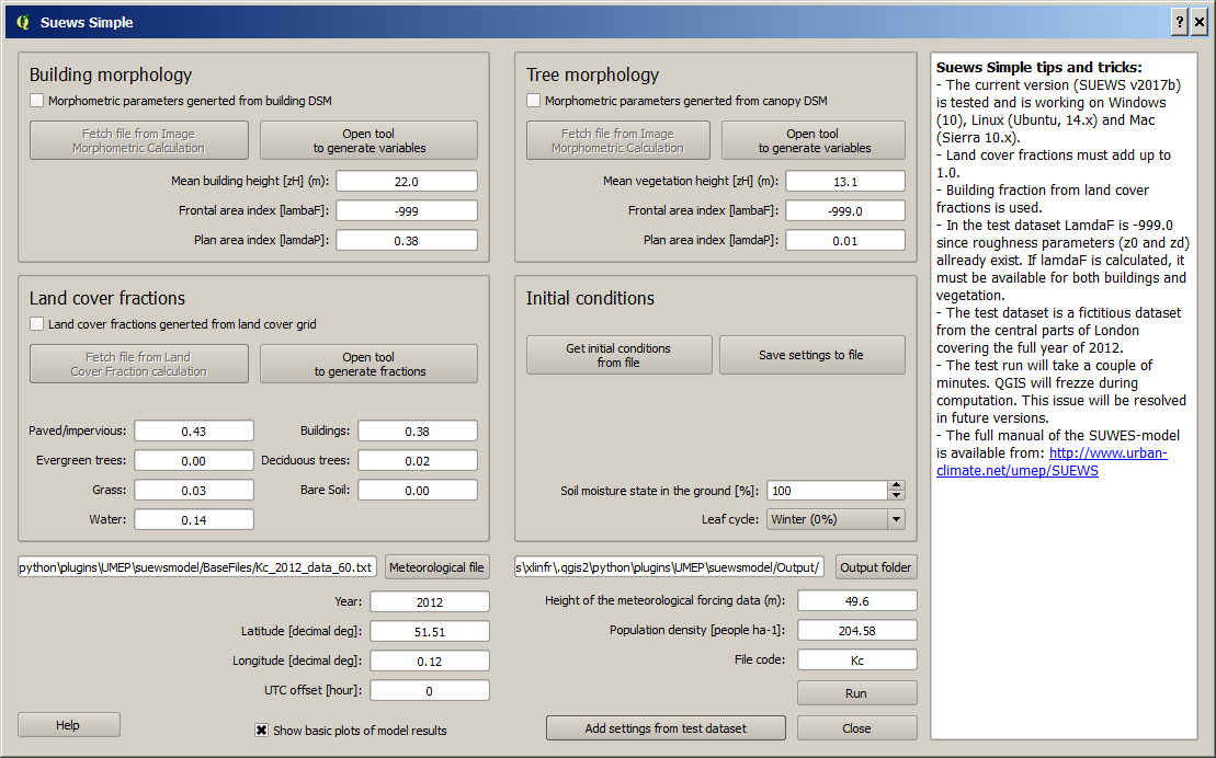
Fig. 9.2 The interface for SUEWS, simple version (click on image to make it larger).
- To make use of this dataset click on Add settings from test dataset (see near bottom of the box). The land cover fractions and all other settings originate from Kotthaus and Grimmond (2014). They used a source area model to obtain the different input parameters (their Fig. 7 in Kotthaus and Grimmond, 2014).
- Before you start the model, change the location of the output data to any location of your choice. Also, make notes on the settings such as Year etc.
- Do a model run and explore the results by clicking Run. A command window appears, when SUEWS performs the calculations using the settings from the interface. Once the calculations are done, some of the results are shown in two summary plots.
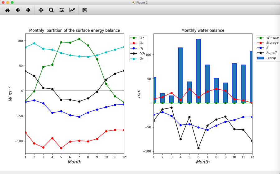
Fig. 9.3 Model output from SUEWS (simple) using the default settings and data (click on image to make it larger).
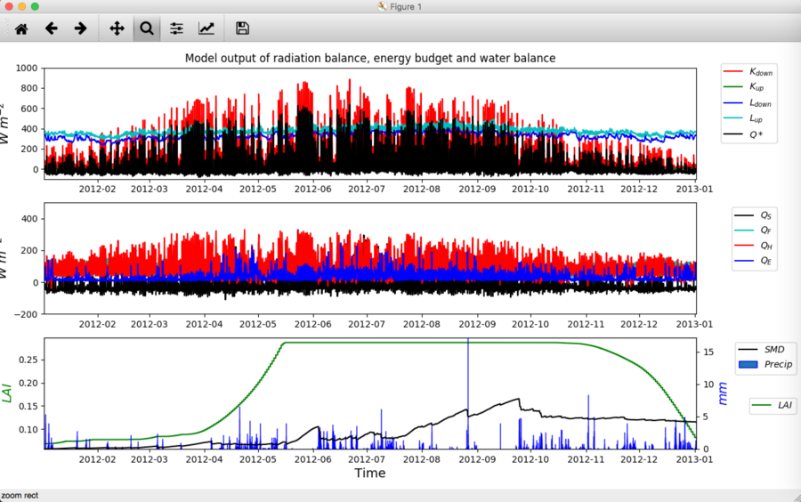
Fig. 9.4 Model output from SUEWS (simple) using the default settings and data (click on image to make it larger).
9.1.6. Model results
The graphs in the upper figure are the monthly mean energy (left) and water balance (right). The lower graphs show the radiation fluxes, energy fluxes, and water related outputs throughout the year. This plot includes a lot of data and it might be difficult to examine it in detail.
To zoom into the plot: use the tools in the top left corner, to zoom to a period of interest. For example, the Zoom in to about the last ten days in March (figure below). This was a period with clear relatively weather.
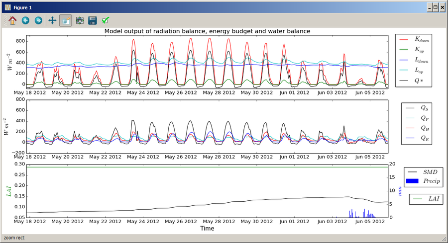
Fig. 9.5 Zoom in on end of March from the daily plot (click on image to make it larger).
9.1.7. Saving a Figure
Use the disk tool in the upper left corner.
- .jpg
- .tif (Recommended)
- .png
9.1.8. Output data Files
In the output folder (you selected earlier) you will find (at least) three files:
- Kc98_2012_60.txt – provides the 60 min model results for site “KC1” for the year 2012
- Kc_FilesChoices.txt – this indicates all options used in the model run see the SUEWS Manual for interpretation of content (this is for when you are doing large number of runs so you know exactly what options were used in each run)
- Kc98_DailyState.txt – this provides the daily mean state (see SUEWS manual for detailed explanation). This allows you to see, for example, the daily state of the LAI (leaf area index).
- Kc_OutputFormat.txt – provides detailed information about the output files such as extended descriptions for each column including units.
If you open these files in a text editor. To understand the header variables read the SUEWS manual.
9.1.9. Sensitivity to land surface fractions
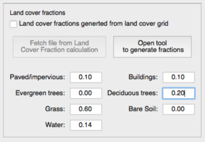
Fig. 9.6 Land cover fractions (click on image to make it larger).
The previous results are for a densely build-up area in London, UK. In order to test the sensitivity of SUEWS to some surface properties you can think about changing some of the surface properties in the SUEWS Simple. For example, change the land cover fraction by:
- Change the land cover fractions as seen in the figure. Feel free to select other values as long as all the fractions add up to 1.0.
- Save the output to a different folder by selecting output folder.
- Click Run.
9.1.10. References
- Grimmond CSB and Oke 1999: Aerodynamic properties of urban areas derived, from analysis of surface form. Journal of Applied Climatology 38:9, 1262-1292
- Grimmond et al. 2015: Climate Science for Service Partnership: China, Shanghai Meteorological Servce, Shanghai, China, August 2015.
- Järvi L, Grimmond CSB & Christen A 2011: The Surface Urban Energy and Water Balance Scheme (SUEWS): Evaluation in Los Angeles and Vancouver J. Hydrol. 411, 219-237
- Järvi L, Grimmond CSB, Taka M, Nordbo A, Setälä H &Strachan IB 2014: Development of the Surface Urban Energy and Water balance Scheme (SUEWS) for cold climate cities, , Geosci. Model Dev. 7, 1691-1711
- Kormann R, Meixner FX 2001: An analytical footprint model for non-neutral stratification. Bound.-Layer Meteorol., 99, 207–224
- Kotthaus S and Grimmond CSB 2014: Energy exchange in a dense urban environment – Part II: Impact of spatial heterogeneity of the surface. Urban Climate 10, 281–307
- Onomura S, Grimmond CSB, Lindberg F, Holmer B, Thorsson S 2015: Meteorological forcing data for urban outdoor thermal comfort models from a coupled convective boundary layer and surface energy balance scheme. Urban Climate. 11:1-23 (link to paper)
- Ward HC, L Järvi, S Onomura, F Lindberg, A Gabey, CSB Grimmond 2016 SUEWS Manual V2016a, http://urban-climate.net/umep/SUEWS Department of Meteorology, University of Reading, Reading, UK
- Ward HC, Kotthaus S, Järvi L and Grimmond CSB 2016b: Surface Urban Energy and Water Balance Scheme (SUEWS): Development and evaluation at two UK sites. Urban Climate http://dx.doi.org/10.1016/j.uclim.2016.05.001
- Ward HC, S Kotthaus, CSB Grimmond, A Bjorkegren, M Wilkinson, WTJ Morrison, JG Evans, JIL Morison, M Iamarino 2015b: Effects of urban density on carbon dioxide exchanges: observations of dense urban, suburban and woodland areas of southern England. Env Pollution 198, 186-200
Authors this document: Lindberg and Grimmond (2016)
9.1.11. Definitions and Notation
To help you find further information about the acronyms they are classified by T: Type of term: C: computer term, S: science term, G: GIS term.
| Definition | T | Ref./Comment | |
|---|---|---|---|
| DEM | Digital elevation model | G | |
| DSM | Digital surface model | G | |
| FAI (λF) | Frontal area index | S | Grimmond and Oke (1999) |
| GUI | Graphical User Interface | C | |
| LAI | Leaf Area Index | S | |
| PAI (λP) | Plan area index | S | |
| png | Portable Network Graphics | C | format for saving plots/figures |
| QGIS | G | www.qgis.org | |
| SUEWS | Surface Urban Energy and Water Balance Scheme | S | |
| Tif | Tagged Image File Format | C | format for saving plots/figures |
| UI | user interface | C | |
| UMEP | Urban Multi-scale Environmental predictor | C | |
| z0 | Roughness length for momentum | S | Grimmond and Oke (1999) |
| zd | Zero plane displacement length for momentum | S | Grimmond and Oke (1999) |
9.1.12. Further explanation
9.1.12.1. Morphometric Methods to determine Roughness parameters:
For more and overview and details see Grimmond and Oke (1999) and Kent et al. (2017a). This uses the height and spacing of roughness elements (e.g. buildings, trees) to model the roughness parameters. For more details see Kent et al. (2017a), Kent et al. (2017b) and [Kent et al. (2017c)]. UMEP has tools for doing this: Pre-processor -> Urban Morphology
9.1.12.2. Source Area Model
For more details see Kotthaus and Grimmond (2014b) and Kent et al. (2017a). The Kormann and Meixner (2001) model is used to determine the probable area that a turbulent flux measurement was impacted by. This is a function of wind direction, stability, turbulence characteristics (friction velocity, variance of the lateral wind velocity) and roughness parameters.